SimaPro and GaBi are the most commonly used software tools to conduct a professional life cycle assessment. There is, however, a third solution in this field, one that is capable of not only calculating product life cycles, but also modeling and improving entire production systems. That integrative solution is called Umberto. While Umberto’s extensive feature list may have initially confused some practitioners in the past, and the interface was sometimes deemed unintuitively technical, let me convince you in this article that the opposite is the actual case now. Especially since the launch of the newest NXT versions, Umberto usability is leaps and bounds ahead of the original, science-derived format. I’ll show you that it now takes not more than one hour to understand the basics and to make your first simple model. You need neither an engineering degree, nor to be an IT geek. All it takes is a computer running a Windows operating system and a small slice of technical common sense.
This tutorial is a concrete guide to working with Umberto. If you are new to material flow modeling and haven’t yet completely understood what this whole life cycle thing is about, you’ll probably enjoy flipping through the blog article How Life Cycle Assessment with LCA Software Works and you might also benefit from understanding Material Flow Based Process Systems Engineering. Why exactly would that be a good idea? Because there are countless examples of how the material flow approach helps not only to assess life cycle related emissions and systematically improve environmental performance, but also to harvest the full potential of efficient manufacturing. Articles on efficient climate control at SWU and more optimization topics shed light on real-life cases. For LCA related uses, check out the article on PVC recycling or red wine carbon footprints. Intrigued?
Download, Install, Create New Project
To start using the free trial of the LCA version, register here and download Umberto NXT LCA. It weighs less than 70 MB and installation is straight-forward. If, instead of trying it on your own, you prefer to watch a professional user show what Umberto is capable of and would like to ask him or her specific questions, you might like to attend one of the web demos that are delivered on a regular basis and are also free. Find the web demo schedule here.
Assuming you successfully downloaded and started the program, you’ll be confronted with a box to enter a serial key. Leave it blank and click OK to start the trial. Next, open the first of three PDF tutorials, at the bottom right of the splash screen. The 24-page-long document gives you a lot more background knowledge that can be quite handy than this rather brief blog article.

Create a new project by choosing File/New/Project and enter a file name. You’re now seeing the “Model” window. It is covered with dots that form a grid. This vast space is where you’ll draw your model. If Umberto were an art class, this window would be your piece of paper. If I were your teacher, I’d now order you to be creative.
Create Process and Inputs
But don’t worry, since we’re just setting up a computer simulation, clicking on the “Add Process” button will suffice for now. In the model toolbar, it is the second button from the left:
This square symbol is the button of choice to make new processes, or transitions, as they used to be called in former versions and in scientific concepts of material flow analysis. Please click on this button first and then anywhere on the white space of the model window. Congratulations, you have just created your first transition. A transition, visualized by a square or rectangle symbol, represents a process. Our new transition bears the name T1, which is quite a sad name and pretty anonymous, so let’s give it a real name. In our example, the model we’re creating is a simplified version of polyethylene production, a common plastic with the abbreviation PE. By clicking on the process name next to the square symbol (“T1”), and then double clicking, a blinking text editing thingy shows up. To name the process, type “PE production” or something similar and then click somewhere else.
Already, we have created the most simple form of a model. But wait a second. Of what use is a model that contains only one process, without any inputs and no outputs? You’re right! It’s pretty pointless. So let’s change this right away. We’ll add two inputs and one output, better sooner than later.
To keep it simple, let’s call the first input “raw materials” and the second one “auxiliary materials”. Press the “Add Input” button in the model toolbar, the one with the green circle.
Let’s draw the first input by clicking somewhere on the dotted space next to the transition. You can name the new input just like you did the “PE production” process. Click on “P1”, now double click on “P1” and type “raw materials”. Next, add the second input (green circle button and a click on the model space again) and call it “auxiliary material”.
If your model shows a vague similarity to this screenshot, you’re on the right track:
Next up, we’ll create an output called “PE granules”. The way to do it is exactly the same as for the inputs, with the only difference now being that you press the red button instead of the green one. The red circle button is used to add outputs to the model. You can drag and drop these input and output places and the transitions anytime you wish to change their positions in the model. You can also drag and drop the names. Play around until it looks nice.
Draw Material Flow Arrows
Now, our model boasts of three places and one process. What else does a material flow model need? Flows, of course! To connect the symbols with each other, we create three flows. One from each input to the process, and one from the process to the output. Select the following button from the model toolbar:
After pressing the arrow button, hover over an input, the green “raw materials” circle for instance, and as the circle turns gray, press the left mouse button and keep it pressed. Drag the arrow to the blue process symbol. Hovering there will make that symbol turn gray, too. Now release the mouse. Congratulations, that’s your first material flow! (Didn’t quite get that? Well, you are in “arrow drawing” mode, because you selected the “Draw Arrow” button. Now imagine you’re moving the input (green circle) to the process (blue square) using drag & drop, as shown in the following screenshot. That’s how you draw an arrow that automatically connects.)
We clearly need two more arrows, one from the second input to the process and another from the process to the output.
Well done. If you move the symbols around, you will see that the arrows automatically adjust. In case they don’t, never mind, something went wrong when drawing the arrows. Just select the arrow, delete it, and draw a new one, this time paying a little more attention to the symbols turning gray.
So far, our model consists of two inputs that lead to a process that, in turn, leads to an output. By now it should look something like this:
Does it? Nice!
Add Material
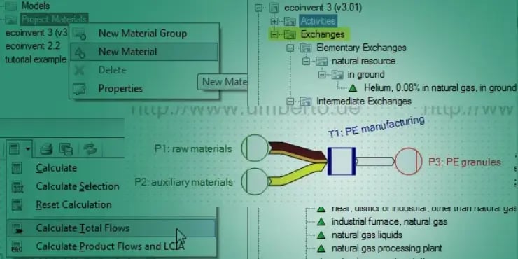
Next up, we feed our model more information on the necessary materials to produce PE. As you can imagine, “raw” and “auxiliary materials” are fairly unspecific, even more so when taking into consideration the claims of sophisticated modeling made by the life cycle assessment approach. Still, to suit the needs of this tutorial, the following rough simplification makes sense. Let’s say that making of PE granulate requires only three input “materials”: crude oil, natural gas and electricity. There are two ways to get these materials into our model. First, we can search for them in the extensive database that comes with Umberto NXT LCA. That database is called ecoinvent 3. You can browse through it in the project explorer (top left corner). To find a material or an activity in the database, type your search term, e.g. “natural gas”, in the project explorer’s search field and click the filter button, as highlighted in the following screenshot.
However, the results for natural gas materials in the exchanges menu are countless. Finding exactly the right material for our example would exceed our tutorial’s scope, so we choose method number two and add a material manually. We just call it plain “natural gas”. Let’s press the New Material button, a triangle with a small green plus, found in the tool bar at the top of the project explorer window:
In the properties window, which pops up at the bottom left corner, type the new material’s name and give it a suitable color. Automatically, each material has a different color, which becomes apparent in the sankey diagram view that we’ll explore further on.
We can add as many materials as we want. We can also add energy, which, for reasons known only to programmers, is also treated as a material in Umberto. When you add the so-called material “electricity”, don’t forget to tell Umberto that electricity is measured in kJ, not in kg. Just like a material’s name and color, its unit is defined in the properties window at the bottom left:
Once you’ve added crude oil, natural gas and electricity, you’ll see these materials show up automatically in the project materials list, with a little green triangle. Look at the project materials folder at the top left, in the project explorer. Found it? Now that you have all necessary input materials, you can start to think about how to specify the process calculation. When you click on the process (the blue square symbol in the model field), you’ll discover two columns appear at the bottom window. The left column lists all relevant inputs, the right one the outputs.
But this is much more than a list. It is the specification of the process, the model’s heart. Let’s add the three materials we’ve just created to the input side. Just drag and drop each material from the project explorer window into the input column, as shown here. Note that the process has to be selected for the specification window to work:
Add all three materials to the process’s input list. Good job.
Set Material Connections
The right column is for the outputs. Oh, well, yes, although we have added an output place, the red circle, we haven’t yet added an output material. Luckily, you know how to do that already, so let’s get it done quickly (it’s the gray little triangle with the little green plus in the project explorer). We’ll call the new material PE granules and add it to the list of the process specs. And as before, we drag the material from the project explorer and drop it in the specification window, only this time, we put it in the output list, the right column. An alternative way to add materials to the process specification, be it as in- or as output, is to press the “Add” button below the list. The window that opens gives you free choice to manually add materials at the top of the list, followed by all options from the ecoinvent database. By the way, for some background information on ecoinvent, check out the Swiss Army Knife of LCA Background Databases.
Two more steps are required for Umberto to know how the materials that we added to the lists interact. First – the easy part – where they come from and where they go. Second, in what quantities and proportions they’re transformed. As we’re still in the specification window, you might wonder why the “Place” column only displays three question marks for each material (“???”). The answer is easy: because the process doesn’t know yet from which place the materials flow. We haven’t specified that yet. Just click on the question marks to do so, to set the respective origin and destination for each material. Crude oil and natural gas are raw materials; they flow from P1:
Electricity is treated as auxiliary material in this example, so select P2 for electricity. The output goes to P3. Easy, wasn’t it? A bit more complicated is how much input creates how much output. As I said, the process lies at the heart of the model. Umberto’s strong point is how flexibly a process can be defined. So what we’ll do, for the sake of keeping it simple, is take a linear specification. So and so much input will generate so and so much output – no scale effects, no dynamic interactions, nothing difficult. In reality, however, no production system quite follows a linear path. That’s why you can also specify Umberto’s processes in four other ways: by almost any mathematical formula, by computer code, with a subnet (a model within a process, see tutorial 3 [Help/Tutorials/…Advanced]), or by loading a predefined process from the module gallery. In our case, we’ll just assume that it takes the same amount of input for each entity we produce, whether we make one kg or thousands of tons of PE granules. After defining some fantasy figures for the coefficients, let’s say 1.1kg crude oil, 0.4 kg natural gas and 1800kJ electricity to give 1 kg of PE granules, we’re almost ready for the calculation. Once you’re getting more familiar with Umberto and are striving for a more precise model (which probably will be the case right after completing this tutorial), you can enter real figures from accounting or from controlling, or from whatever source you wish. You don’t need to calculate the coefficient, just enter the plain numbers, Umberto will do the rest. Did you watch your clock? Wasn’t that difficult, was it?
Calculate!
Well, there is one last task to fulfill before doing the calculation. This is called setting the manual flow. We’re basically telling Umberto the quantity for which we would like to see the results. That can be the functional unit of the LCA, e.g., one kg of PE granules, or the entire annual production of the process we modeled. Click on the arrow that leads to the red PE granules output place. The window at the bottom of the program will now display the arrow specifications, similar to the process specs we dealt with before. Let’s add “PE granules” to the specs. Like the process materials, we can either add a material to the arrow specs by drag and drop (move the PE granules from the project materials (project explorer window) into the arrow specification window), or by clicking the green plus button below the specifications and selecting PE granules from the list. In the quantity column, enter 1 kg. Note how the arrow turns from gray to purple, indicating that this arrow now contains the manual flow. That’s it! We can calculate the model!
Next to the calculator symbol (in the model toolbar) there is a tiny black triangle. Pushing it will give you a choice of possible calculations. “Total flows” is what we need:
Umberto now calculates results from our model, which shouldn’t take any longer than a few milliseconds. When that is done, try clicking the model toolbar button that looks like a little flag. This is the button that toggles the Sankey diagram view:
If you followed the instructions thoroughly, your model will look something like this.
Mind, I tweaked the looks by playing around with the color and the angle of the labels, and I slightly changed the arrow properties, too. Click an arrow or a text label and explore the possibilities in the properties window at the bottom left. Concerning the arrows, try ticking “Rounded”, and set the curviness to at least 50 px for a much smoother looking model in Sankey view. We should never underestimate the importance of aesthetics in information transfer – elegant sankey diagrams are powerful tools.
Congratulations for your first material flow model! You’re getting very close to obtaining real results with more precise models. Just dive into the tutorials shipped with the program, sign up for a free online demo delivered by an expert or check out the forum or the downloads, accessible via Umberto’s help menu or the links below.
With the modeling skills that you’re now familiar with, you can easily work through Tutorial 2 and grasp all the necessary information needed to use the database and understand impact assessment, the soul of LCA, the thing that makes life cycle assessment such an interesting method.
Welcome to the club and happy life cycling!
Links
- Download Umberto NXT LCA (14-day trial version, free registration required)
- Get behind some LCAs and process optimization decisions conducted with Umberto
- Insights from user workshops (free registration required)
Article image CC by Moritz Bühner